RR Skills (2): Graph Production

November 4, 2014

Overview of the Series

Oct 14 – Intro to Reproducible Research
Oct 21 – RR Basic Skills (1): Data Manipulation
Oct 28 – Intro to Latent Class and Latent Transition Models
Nov 4 – RR Basic Skills (2): Graph Production
Nov 11
Nov 18 – RR Basic Skills (3): Statistical Modeling
Nov 25 – RR Basic Skills (4): Dynamic Reporting
Dec 2 – Migrating into R from other Statistical Software

Previously:

Tidy data

Each variable forms a column
Each observation forms a row
Each type of observational unit forms a table

Previously:

"./Scripts/Data/dsL.R"

download the files to work along at GitHub

Previously:

"./Scripts/Data/dsL.R"

imported the raw data files

myExtract <- "./Data/Extract/NLSY97_Attend_20141021/NLSY97_Attend_20141021"
pathSourceData <- paste0(myExtract,".csv") 
SourceData <- read.csv(pathSourceData,header=TRUE, skip=0,sep=",")
ds0 <- SourceData

cleaned, transformed , and at the end, exported it.

pathdsLrds <- "./Data/Derived/dsL.rds"
saveRDS(object=dsL, file=pathdsLrds, compress="xz")

The slides on data manipulation were in fact annotations over the live script ./Scripts/Data/dsL.R that brings data to the "dsL" stage every time it is sourced.

Load Data

# loads basic NLSY97-religiosity data as defined in COAG-Colloquium-2014F repository
source("./Scripts/Data/dsL.R")

str(dsL)

'data.frame':   107772 obs. of  12 variables:
 $ id     : int  1 1 1 1 1 1 1 1 1 1 ...
 $ sex    : int  2 2 2 2 2 2 2 2 2 2 ...
 $ race   : int  4 4 4 4 4 4 4 4 4 4 ...
 $ bmonth : int  9 9 9 9 9 9 9 9 9 9 ...
 $ byear  : int  1981 1981 1981 1981 1981 1981 1981 1981 1981 1981 ...
 $ year   : int  2000 2001 2002 2003 2004 2005 2006 2007 2008 2009 ...
 $ attend : int  1 6 2 1 1 1 1 1 1 1 ...
 $ age    : int  19 20 21 22 23 24 25 26 27 28 ...
 $ sexF   : Ord.factor w/ 3 levels "Male"<"Female"<..: 2 2 2 2 2 2 2 2 2 2 ...
 $ raceF  : Ord.factor w/ 4 levels "Black"<"Hispanic"<..: 4 4 4 4 4 4 4 4 4 4 ...
 $ bmonthF: Ord.factor w/ 12 levels "Jan"<"Feb"<"Mar"<..: 9 9 9 9 9 9 9 9 9 9 ...
 $ attendF: Ord.factor w/ 8 levels "Never"<"Once or Twice"<..: 1 6 2 1 1 1 1 1 1 1 ...

Load Data

# loads basic NLSY97-religiosity data as defined in COAG-Colloquium-2014F repository
source("./Scripts/Data/dsL.R")

str(dsL)

'data.frame':   107772 obs. of  12 variables:
 $ id     : int  1 1 1 1 1 1 1 1 1 1 ...
 $ sex    : int  2 2 2 2 2 2 2 2 2 2 ...
 $ race   : int  4 4 4 4 4 4 4 4 4 4 ...
 $ bmonth : int  9 9 9 9 9 9 9 9 9 9 ...
 $ byear  : int  1981 1981 1981 1981 1981 1981 1981 1981 1981 1981 ...
 $ year   : int  2000 2001 2002 2003 2004 2005 2006 2007 2008 2009 ...
 $ attend : int  1 6 2 1 1 1 1 1 1 1 ...
 $ age    : int  19 20 21 22 23 24 25 26 27 28 ...
 $ sexF   : Ord.factor w/ 3 levels "Male"<"Female"<..: 2 2 2 2 2 2 2 2 2 2 ...
 $ raceF  : Ord.factor w/ 4 levels "Black"<"Hispanic"<..: 4 4 4 4 4 4 4 4 4 4 ...
 $ bmonthF: Ord.factor w/ 12 levels "Jan"<"Feb"<"Mar"<..: 9 9 9 9 9 9 9 9 9 9 ...
 $ attendF: Ord.factor w/ 8 levels "Never"<"Once or Twice"<..: 1 6 2 1 1 1 1 1 1 1 ...

Load Data

dplyr::filter(dsL, id==1)

   id sex race bmonth byear year attend age   sexF       raceF bmonthF         attendF
1   1   2    4      9  1981 2000      1  19 Female Non-B/Non-H     Sep           Never
2   1   2    4      9  1981 2001      6  20 Female Non-B/Non-H     Sep About once/week
3   1   2    4      9  1981 2002      2  21 Female Non-B/Non-H     Sep   Once or Twice
4   1   2    4      9  1981 2003      1  22 Female Non-B/Non-H     Sep           Never
5   1   2    4      9  1981 2004      1  23 Female Non-B/Non-H     Sep           Never
6   1   2    4      9  1981 2005      1  24 Female Non-B/Non-H     Sep           Never
7   1   2    4      9  1981 2006      1  25 Female Non-B/Non-H     Sep           Never
8   1   2    4      9  1981 2007      1  26 Female Non-B/Non-H     Sep           Never
9   1   2    4      9  1981 2008      1  27 Female Non-B/Non-H     Sep           Never
10  1   2    4      9  1981 2009      1  28 Female Non-B/Non-H     Sep           Never
11  1   2    4      9  1981 2010      1  29 Female Non-B/Non-H     Sep           Never
12  1   2    4      9  1981 2011      1  30 Female Non-B/Non-H     Sep           Never

Load Data

dplyr::filter(dsL, id==1) %>% select(id, year, attend, attendF, sexF, raceF)

   id year attend         attendF   sexF       raceF
1   1 2000      1           Never Female Non-B/Non-H
2   1 2001      6 About once/week Female Non-B/Non-H
3   1 2002      2   Once or Twice Female Non-B/Non-H
4   1 2003      1           Never Female Non-B/Non-H
5   1 2004      1           Never Female Non-B/Non-H
6   1 2005      1           Never Female Non-B/Non-H
7   1 2006      1           Never Female Non-B/Non-H
8   1 2007      1           Never Female Non-B/Non-H
9   1 2008      1           Never Female Non-B/Non-H
10  1 2009      1           Never Female Non-B/Non-H
11  1 2010      1           Never Female Non-B/Non-H
12  1 2011      1           Never Female Non-B/Non-H

Today's objective

Minimalistic start

dplyr::filter(dsL, id==1) %>% 
  dplyr::select(id, year, attend, attendF)

   id year attend         attendF
1   1 2000      1           Never
2   1 2001      6 About once/week
3   1 2002      2   Once or Twice
4   1 2003      1           Never
5   1 2004      1           Never
6   1 2005      1           Never
7   1 2006      1           Never
8   1 2007      1           Never
9   1 2008      1           Never
10  1 2009      1           Never
11  1 2010      1           Never
12  1 2011      1           Never

How often did you attend a worhsip service during the last year?

  attendLevels         attendLabels
1            8             Everyday
2            7   Several times/week
3            6      About once/week
4            5    About twice/month
5            4     About once/month
6            3 Less than once/month
7            2        Once or Twice
8            1                Never

Q: How do we map these data to abstract dimensions?

Preparing the canvas

dsM <- dplyr::filter(dsL, id == 1) %>% 
  dplyr::select(id, year, attend, attendF)
dsM

   id year attend         attendF
1   1 2000      1           Never
2   1 2001      6 About once/week
3   1 2002      2   Once or Twice
4   1 2003      1           Never
5   1 2004      1           Never
6   1 2005      1           Never
7   1 2006      1           Never
8   1 2007      1           Never
9   1 2008      1           Never
10  1 2009      1           Never
11  1 2010      1           Never
12  1 2011      1           Never

p <- ggplot2::ggplot(dsM,aes(x=year,y=attend))
p

# Error: No layers in plot

Next: add a geom
Note: Data mapping

First strokes: points

dsM <- dplyr::filter(dsL, id == 1) %>% 
  dplyr::select(id, year, attend, attendF)
dsM

   id year attend         attendF
1   1 2000      1           Never
2   1 2001      6 About once/week
3   1 2002      2   Once or Twice
4   1 2003      1           Never
5   1 2004      1           Never
6   1 2005      1           Never
7   1 2006      1           Never
8   1 2007      1           Never
9   1 2008      1           Never
10  1 2009      1           Never
11  1 2010      1           Never
12  1 2011      1           Never

p <- ggplot2::ggplot(dsM,aes(x=year,y=attend))
p <- p + geom_point()

p

Note: Geom
Next: try a different geom

First strokes: lines

dsM <- dplyr::filter(dsL, id == 1) %>% 
  dplyr::select(id, year, attend, attendF)
dsM

   id year attend         attendF
1   1 2000      1           Never
2   1 2001      6 About once/week
3   1 2002      2   Once or Twice
4   1 2003      1           Never
5   1 2004      1           Never
6   1 2005      1           Never
7   1 2006      1           Never
8   1 2007      1           Never
9   1 2008      1           Never
10  1 2009      1           Never
11  1 2010      1           Never
12  1 2011      1           Never

p <- ggplot2::ggplot(dsM,aes(x=year,y=attend))
p <- p + geom_line()

p

Note: list of geoms
Next: combine geoms

First strokes

dsM <- dplyr::filter(dsL, id == 1) %>% 
  dplyr::select(id, year, attend, attendF)
dsM

   id year attend         attendF
1   1 2000      1           Never
2   1 2001      6 About once/week
3   1 2002      2   Once or Twice
4   1 2003      1           Never
5   1 2004      1           Never
6   1 2005      1           Never
7   1 2006      1           Never
8   1 2007      1           Never
9   1 2008      1           Never
10  1 2009      1           Never
11  1 2010      1           Never
12  1 2011      1           Never

p <- ggplot2::ggplot(dsM,aes(x=year,y=attend))
p <- p + geom_line()
p <- p + geom_point()
p

Next: mapping inside geoms

Flexible mapping

dsM <- dplyr::filter(dsL, id == 1) %>% 
  dplyr::select(id, year, attend, attendF)
dsM

   id year attend         attendF
1   1 2000      1           Never
2   1 2001      6 About once/week
3   1 2002      2   Once or Twice
4   1 2003      1           Never
5   1 2004      1           Never
6   1 2005      1           Never
7   1 2006      1           Never
8   1 2007      1           Never
9   1 2008      1           Never
10  1 2009      1           Never
11  1 2010      1           Never
12  1 2011      1           Never

p <- ggplot2::ggplot(dsM,aes(x=year))
p <- p + geom_line(aes(y=attend))
p <- p + geom_point(aes(y=attend))
p

Next: custom graphical themes

Flexibility of styling

baseSize <- 12
plotTheme <- ggplot2::theme_bw() +
  ggplot2::theme_bw(base_size=baseSize)+
  ggplot2::theme(title=ggplot2::element_text(colour="gray20",size = baseSize + 3)) +
  ggplot2::theme(axis.text=ggplot2::element_text(colour="gray40", size= baseSize - 2))+
  ggplot2::theme(axis.title.x=ggplot2::element_text(colour="gray40", size = baseSize + 2, vjust=-.3))+
  ggplot2::theme(axis.title.y=ggplot2::element_text(colour="gray40", size = baseSize + 2, vjust=1.3))+
  ggplot2::theme(panel.border = ggplot2::element_rect(colour="gray80"))+
  ggplot2::theme(axis.ticks.length = grid::unit(0, "cm"))

Next: apply theme

Theme vs No Theme

p <- ggplot2::ggplot(dsM,aes(x=year,y=attend))
p <- p + geom_line()
p <- p + geom_point()
p <- p + plotTheme
p

plot of chunk graph05 Note: more theme options
Next: scales, setting axis range

p <- ggplot2::ggplot(dsM,aes(x=year))
p <- p + geom_line(aes(y=attend))
p <- p + geom_point(aes(y=attend))

p

Customizing scales: X : limits

p <- ggplot2::ggplot(dsM,aes(x=year,y=attend))
p <- p + geom_line()
p <- p + geom_point()
p <- p + plotTheme
p <- p + scale_x_continuous(limits=c(1995,2015))
p

plot of chunk graph06

p <- ggplot2::ggplot(dsM,aes(x=year,y=attend))
p <- p + geom_line()
p <- p + geom_point()
p <- p + plotTheme

p

Note: Scales
Next: set axis breaks

Customizing scales: X : breaks

p <- ggplot2::ggplot(dsM,aes(x=year,y=attend))
p <- p + geom_line()
p <- p + geom_point()
p <- p + plotTheme
p <- p + scale_x_continuous(limits=c(2000,2011),
                            breaks=c(2000:2011))
p

plot of chunk graph07

p <- ggplot2::ggplot(dsM,aes(x=year,y=attend))
p <- p + geom_line()
p <- p + geom_point()
p <- p + plotTheme
p <- p + scale_x_continuous(limits=c(1995,2015))

p

plot of chunk graph06a Next: breaks customization

Customizing scales: X : breaks : manual

p <- ggplot2::ggplot(dsM,aes(x=year,y=attend))
p <- p + geom_line()
p <- p + geom_point()
p <- p + plotTheme
p <- p + scale_x_continuous(limits=c(2000,2011),
                            breaks=c(2000,2005,2010))
p

plot of chunk graph08

p <- ggplot2::ggplot(dsM,aes(x=year,y=attend))
p <- p + geom_line()
p <- p + geom_point()
p <- p + plotTheme
p <- p + scale_x_continuous(limits=c(1995,2015))

p

plot of chunk graph06a Next: customizing y-axis

Customizing scales: Y

p <- ggplot2::ggplot(dsM,aes(x=year,y=attend))
p <- p + geom_line()
p <- p + geom_point()
p <- p + plotTheme
p <- p + scale_x_continuous(limits=c(2000,2011),
                            breaks=c(2000:2011))
p

Next: with y-axis customized

Customizing scales: Y

p <- ggplot2::ggplot(dsM,aes(x=year,y=attend))
p <- p + geom_line()
p <- p + geom_point()
p <- p + plotTheme
p <- p + scale_x_continuous(limits=c(2000,2011),
                            breaks=c(2000:2011))
p <- p + scale_y_continuous(limits=c(1,8),
                            breaks=seq(1,8, by=1))
p

Next: axes titles

Customizing scales: Y

p <- ggplot2::ggplot(dsM,aes(x=year,y=attend))
p <- p + geom_line()
p <- p + geom_point()
p <- p + plotTheme
p <- p + scale_x_continuous(limits=c(2000,2011),
                            breaks=c(2000:2011))
p <- p + scale_y_continuous(limits=c(1,8),
                            breaks=seq(2,8, by=2))
p

Next: axes titles

Axes titles

p <- ggplot2::ggplot(dsM,aes(x=year,y=attend))
p <- p + geom_line()
p <- p + geom_point()
p <- p + plotTheme
p <- p + scale_x_continuous(limits=c(2000,2011),
                            breaks=c(2000:2011),
                            "Year of observation")
p <- p + scale_y_continuous(limits=c(1,8),
                            breaks=seq(1,8, by=1),
                            "Church attendance")
p

Next: adding main title

Main title

p <- ggplot2::ggplot(dsM,aes(x=year,y=attend))
p <- p + geom_line()
p <- p + geom_point()
p <- p + plotTheme
p <- p + scale_x_continuous(limits=c(2000,2011),
                            breaks=c(2000:2011),
                            "Year of observation")
p <- p + scale_y_continuous(limits=c(1,8),
                            breaks=seq(1,8, by=1),
                            "Church attendance")
p <- p + ggtitle(
  "How frequently did you attend worship last year?")
p

Next: learning the lingo
Note: alternatives, cheatsheet

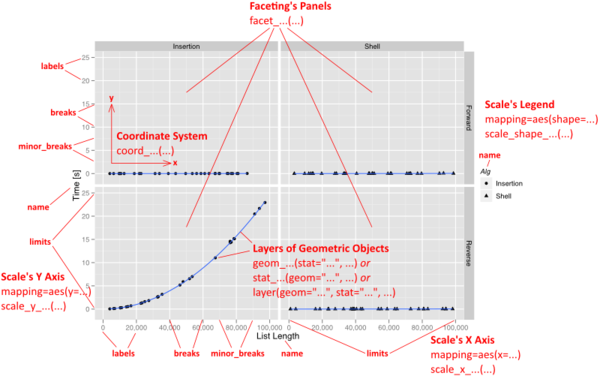
The anatomy of a ggplot

The names of ggplot elements are visually explained in another great ggplot quick reference by SAPE research group.

Next: adding units

Minimalistic + 1

dsM <- dplyr::filter(dsL, id %in% c(1,23)) %>% 
  dplyr::select(id, year, attend, attendF)
#
p <- ggplot2::ggplot(dsM,aes(x=year,y=attend))
p <- p + geom_line()
p <- p + geom_point()
p <- p + plotTheme
p <- p + scale_x_continuous(limits=c(2000,2011),
                            breaks=c(2000:2011))
p <- p + scale_y_continuous(limits=c(1,8), 
                            breaks=seq(1,8, by=1))
p <- p + labs(list(
  title="How often did you attend worship last year?",
  x="Year of observation", y="Church attendance"))
p

plot of chunk graph12

Next: grouping cases

Map groupings : individuals

dsM <- dplyr::filter(dsL, id %in% c(1,23)) %>% 
  dplyr::select(id, year, attend, attendF)
#
p <- ggplot2::ggplot(dsM,aes(x=year,y=attend))
p <- p + geom_line(aes(group=id))
p <- p + geom_point()
p <- p + plotTheme
p <- p + scale_x_continuous(limits=c(2000,2011),
                            breaks=c(2000:2011))
p <- p + scale_y_continuous(limits=c(1,8), 
                            breaks=seq(1,8, by=1))
p <- p + labs(list(
  title="How often did you attend worship last year?",
  x="Year of observation", y="Church attendance"))
p

Next: adding more cases

Facing the Overplotting Issue

dsM <- dplyr::filter(dsL, id <=300) %>% 
  dplyr::select(id, year, attend, attendF)
#  
p <- ggplot2::ggplot(dsM,aes(x=year,y=attend))
p <- p + geom_line(aes(group=id))
p <- p + geom_point()
p <- p + plotTheme
p <- p + scale_x_continuous(limits=c(2000,2011),
                            breaks=c(2000:2011))
p <- p + scale_y_continuous(limits=c(1,8), 
                            breaks=seq(1,8, by=1))
p <- p + labs(list(
  title="How often did you attend worship last year?",
  x="Year of observation", y="Church attendance"))
p

Next: jittering lines
Note: press "p" for zoom

Jittering lines

dsM <- dplyr::filter(dsL, id <=300) %>% 
  dplyr::select(id, year, attend, attendF)
#  
p <- ggplot2::ggplot(dsM,aes(x=year,y=attend))
p <- p + geom_line(aes(group=id), 
           position=position_jitter(w=0.3,h=0.3))
p <- p + geom_point()
p <- p + plotTheme
p <- p + scale_x_continuous(limits=c(2000,2011),
                            breaks=c(2000:2011))
p <- p + scale_y_continuous(limits=c(0,8), 
                            breaks=seq(1,8, by=1))
p <- p + labs(list(
  title="How often did you attend worship last year?",
  x="Year of observation", y="Church attendance"))
p

plot of chunk graph15

Next: jittering points
Note: press "p" for zoom

Jittering points

dsM <- dplyr::filter(dsL, id <=300) %>% 
  dplyr::select(id, year, attend, attendF)
#  
p <- ggplot2::ggplot(dsM,aes(x=year,y=attend))
p <- p + geom_line(aes(group=id), 
           position=position_jitter(w=0.3, h=0.3))
p <- p + geom_point(
           position=position_jitter(w=0.3, h=0.3))
p <- p + plotTheme
p <- p + scale_x_continuous(limits=c(2000,2011),
                            breaks=c(2000:2011))
p <- p + scale_y_continuous(limits=c(0,8), 
                            breaks=seq(1,8, by=1))
p <- p + labs(list(
  title="How often did you attend worship last year?",
  x="Year of observation", y="Church attendance"))
p

plot of chunk graph16

Next: coloring lines
Note: press "p" for zoom

Coloring lines

dsM <- dplyr::filter(dsL, id <=300) %>% 
  dplyr::select(id, year, attend, attendF)
p <- ggplot2::ggplot(dsM,aes(x=year,y=attend))
#  
p <- p + geom_line(aes(group=id), color='firebrick',
           position=position_jitter(w=0.3, h=0.3))
p <- p + geom_point(
           position=position_jitter(w=0.3, h=0.3))
p <- p + plotTheme
p <- p + scale_x_continuous(limits=c(2000,2011),
                            breaks=c(2000:2011))
p <- p + scale_y_continuous(limits=c(0,8), 
                            breaks=seq(1,8, by=1))
p <- p + labs(list(
  title="How often did you attend worship last year?",
  x="Year of observation", y="Church attendance"))
p

plot of chunk graph17

Next: coloring points
Note: press "p" for zoom

To use human names for colors, refer to the [R color palette](colors in R. For explore computer palette colrd.org and colorbrewer2

Coloring points

dsM <- dplyr::filter(dsL, id <=300) %>% 
  dplyr::select(id, year, attend, attendF)
#  
p <- ggplot2::ggplot(dsM,aes(x=year,y=attend))
p <- p + geom_line(aes(group=id), color='firebrick',
           position=position_jitter(w=0.3, h=0.3))
p <- p + geom_point(shape=21, color=NA, fill="blue4",
           position=position_jitter(w=0.3, h=0.3))
p <- p + plotTheme
p <- p + scale_x_continuous(limits=c(2000,2011),
                            breaks=c(2000:2011))
p <- p + scale_y_continuous(limits=c(0,8), 
                            breaks=seq(1,8, by=1))
p <- p + labs(list(
  title="How often did you attend worship last year?",
  x="Year of observation", y="Church attendance"))
p

plot of chunk graph18

Next: alpha
Note: press "p" for zoom

For shape and linetypes consult R cookbook or SAPE Quick Reference

Transparancy / Alpha channel

dsM <- dplyr::filter(dsL, id <=300) %>% 
  dplyr::select(id, year, attend, attendF)
#  
p <- ggplot2::ggplot(dsM,aes(x=year,y=attend))
p <- p + geom_line(aes(group=id), color='firebrick',
           alpha=.3,
           position=position_jitter(w=0.3, h=0.3))
p <- p + geom_point(shape=21, color=NA, fill="blue4",
           alpha=.3, 
           position=position_jitter(w=0.3, h=0.3))
p <- p + plotTheme
p <- p + scale_x_continuous(limits=c(2000,2011),
                            breaks=c(2000:2011))
p <- p + scale_y_continuous(limits=c(0,8), 
                            breaks=seq(1,8, by=1))
p <- p + labs(list(
  title="How often did you attend worship last year?",
  x="Year of observation", y="Church attendance"))
p

plot of chunk graph19

Next: tuning 1
Note: press "p" for zoom

Fainter, larger dots

dsM <- dplyr::filter(dsL, id <=300) %>% 
  dplyr::select(id, year, attend, attendF)
#  
p <- ggplot2::ggplot(dsM,aes(x=year,y=attend))
p <- p + geom_line(aes(group=id), color='firebrick',
           alpha=.1,
           position=position_jitter(w=0.3, h=0.3))
p <- p + geom_point(shape=21, color=NA, fill="blue4",
           alpha=.2, size=2.2, 
           position=position_jitter(w=0.3, h=0.3))
p <- p + plotTheme
p <- p + scale_x_continuous(limits=c(2000,2011),
                            breaks=c(2000:2011))
p <- p + scale_y_continuous(limits=c(0,8), 
                            breaks=seq(1,8, by=1))
p <- p + labs(list(
  title="How often did you attend worship last year?",
  x="Year of observation", y="Church attendance"))
p

Next: tuning 2
Note: press "p" for zoom

Crisper, smaller dots

dsM <- dplyr::filter(dsL, id <=300) %>% 
  dplyr::select(id, year, attend, attendF)
#  
p <- ggplot2::ggplot(dsM,aes(x=year,y=attend))
p <- p + geom_line(aes(group=id), color='firebrick',
           alpha=.1,
           position=position_jitter(w=0.3, h=0.3))
p <- p + geom_point(shape=21, color=NA, fill="blue4",
           alpha=.5, size=.8, 
           position=position_jitter(w=0.3, h=0.3))
p <- p + plotTheme
p <- p + scale_x_continuous(limits=c(2000,2011),
                            breaks=c(2000:2011))
p <- p + scale_y_continuous(limits=c(0,8), 
                            breaks=seq(1,8, by=1))
p <- p + labs(list(
  title="How often did you attend worship last year?",
  x="Year of observation", y="Church attendance"))
p

Next: faceting 1
Note: press "p" for zoom

Faceting

dsM <- dplyr::filter(dsL, id <=300) %>% 
  dplyr::select(id, sexF, raceF, year, attend, attendF)
#  
p <- ggplot2::ggplot(dsM,aes(x=year,y=attend))
p <- p + geom_line(aes(group=id), color='firebrick',
           alpha=.1,
           position=position_jitter(w=0.3, h=0.3))
p <- p + geom_point(shape=21, color=NA, fill="blue4",
           alpha=.3, size=1.2, 
           position=position_jitter(w=0.3, h=0.3))
p <- p + plotTheme
p <- p + scale_x_continuous(limits=c(2000,2011),
                            breaks=c(2000:2011))
p <- p + scale_y_continuous(limits=c(0,8), 
                            breaks=seq(1,8, by=1))
p <- p + labs(list(
  title="How often did you attend worship last year?",
  x="Year of observation", y="Church attendance"))
p <- p + facet_grid(sexF~raceF)
p

plot of chunk graph22

Next: removing factor level
Note: press "p" for zoom

Exclude levels

dsM <- dplyr::filter(dsL, id <=300, 
                     raceF != "Mixed (Non-H)") %>% 
  dplyr::select(id, sexF, raceF, year, attend, attendF)
#  
p <- ggplot2::ggplot(dsM,aes(x=year,y=attend))
p <- p + geom_line(aes(group=id), color='firebrick',
           alpha=.1,
           position=position_jitter(w=0.3, h=0.3))
p <- p + geom_point(shape=21, color=NA, fill="blue4",
                    alpha=.5, size=.8, 
                    position=position_jitter(w=0.3, h=0.3))
p <- p + plotTheme
p <- p + scale_x_continuous(limits=c(2000,2011),
                            breaks=c(2000:2011))
p <- p + scale_y_continuous(limits=c(0,8), 
                            breaks=seq(1,8, by=1))
p <- p + labs(list(
  title="How often did you attend worship last year?",
  x="Year of observation", y="Church attendance"))
p <- p + facet_grid(sexF~raceF)
p

plot of chunk graph23

Next: tranforming variable
Note: press "p" for zoom

Centering time

dsM <- dplyr::filter(dsL, id <=300, 
                     raceF != "Mixed (Non-H)") %>% 
  dplyr::select(id, sexF, raceF, year, attend, attendF) %>%
  dplyr::mutate(yearc = year - 2000)
#  
p <- ggplot2::ggplot(dsM,aes(x=yearc,y=attend))
p <- p + geom_line(aes(group=id), color='firebrick',
           alpha=.1,
           position=position_jitter(w=0.3, h=0.3))
p <- p + geom_point(shape=21, color=NA, fill="blue4",
           alpha=.5, size=.8, 
           position=position_jitter(w=0.3, h=0.3))
p <- p + plotTheme
p <- p + scale_x_continuous(limits=c(0,11),
                            breaks=c(0:11))
p <- p + scale_y_continuous(limits=c(0,8), 
                            breaks=seq(1,8, by=1))
p <- p + labs(list(
  title="How often did you attend worship last year?",
  x="Years since 2000", y="Church attendance"))
p <- p + facet_grid(sexF~raceF)
p

plot of chunk graph24

Next: final styling
Note: press "p" for zoom

Final touches

dsM <- dplyr::filter(dsL, id <=300, 
                     raceF != "Mixed (Non-H)") %>% 
  dplyr::select(id, sexF, raceF, year, attend, attendF) %>%
  dplyr::mutate(yearc = year - 2000)
#  
p <- ggplot2::ggplot(dsM,aes(x=yearc,y=attend))
p <- p + geom_line(aes(group=id), color='firebrick',
           alpha=.2,
           position=position_jitter(w=0.3, h=0.3))
p <- p + geom_point(shape=21, color=NA, fill="blue4",
           alpha=.4, size=1, 
           position=position_jitter(w=0.3, h=0.3))
p <- p + plotTheme
p <- p + scale_x_continuous(limits=c(0,11),
                            breaks=c(0:11))
p <- p + scale_y_continuous(limits=c(0,8), 
                            breaks=seq(1,8, by=1))
p <- p + labs(list(
  title="How often did you attend worship last year?",
  x="Years since 2000", y="Church attendance"))
p <- p + facet_grid(sexF~raceF)
p

.

Next: final graph

Next time

Oct 14 – Intro to Reproducible Research
Oct 21 – RR Basic Skills (1): Data Manipulation
Oct 28 – Intro to Latent Class and Latent Transition Models
Nov 4 – RR Basic Skills (2): Graph Production
Nov 11
Nov 18 – RR Basic Skills (3): Statistical Modeling
Nov 25 – RR Basic Skills (4): Dynamic Reporting
Dec 2 – Migrating into R from other Statistical Software

Question? Comments?

You can forward questions to Ann Greenwood (ann.greenwood@popdata.bc.ca) or Vincenza Gruppuso (vincenza@uvic.ca) during the live Q&A. They are standing by to take your questions.